Using Unified Architecture Framework (UAF) for a Space Mission Modelling
Accelerate Systems Design
Introduction
This article explores the application of the Unified Architecture Framework (UAF) in the context of aerospace, specifically focusing on mission engineering for a Mars Exploration and Sample Return mission.
With the increasing complexity of space missions, the need for a robust framework that can manage various interrelated systems and organizations is more critical than ever. UAF, with its specialized viewpoints and elements, offers a structured approach to modeling Systems of Systems (SoS), ensuring that all aspects of the mission are aligned with the broader strategic objectives.
Systems of Systems definition (SoS) according to INCOSE Systems Engineering Handbook Edition 5:
A set of systems or system elements that interact to provide a unique capability that none of the constituent systems can accomplish on its own.
To perform mission analysis, it is crucial to define the different aspects, including strategic goals for the overall mission, expected capabilities, different phases and steps, expected tasks to be performed and interactions between different the systems and the human operators needed to achieve the expected capabilities at the mission level.
UAF Standard
Overview of UAF standard
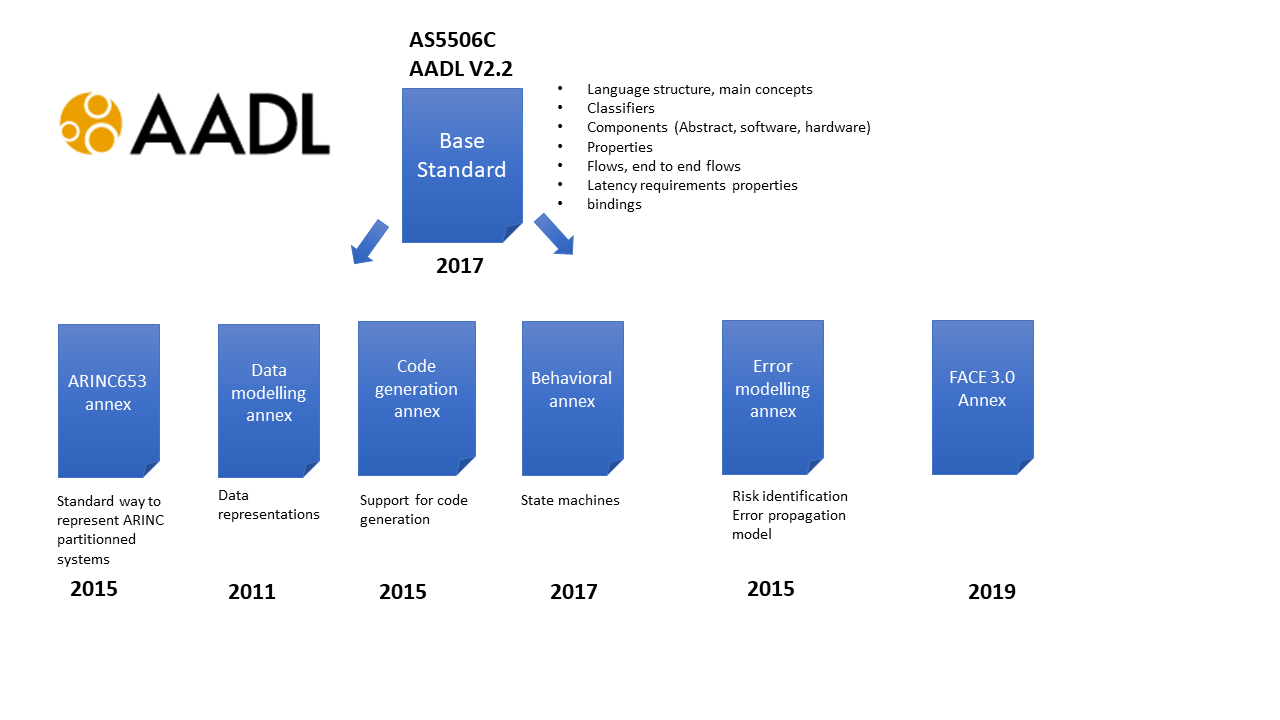
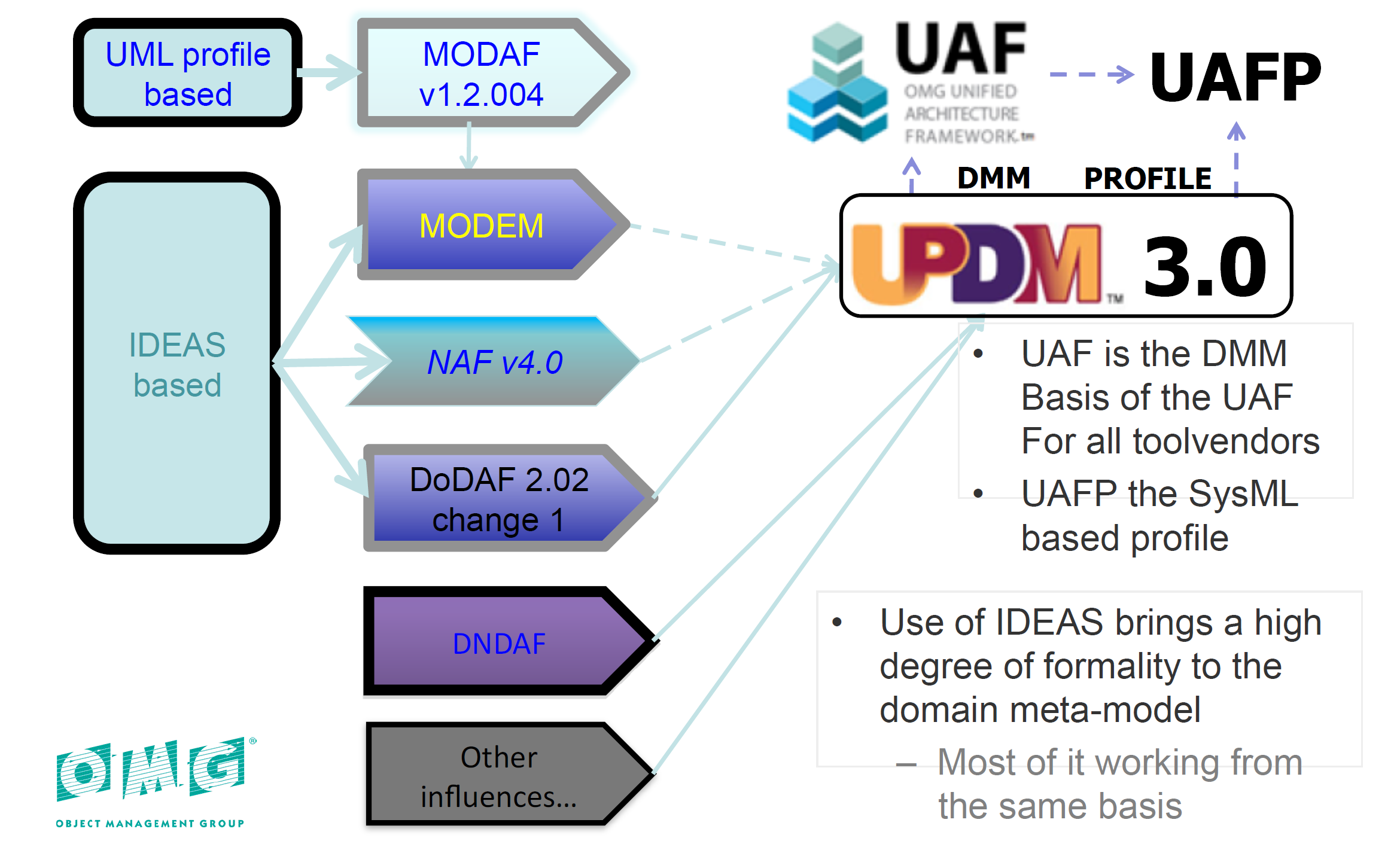
The Unified Architecture Framework (UAF) is an architecture framework proposed by the Object Management Group (OMG). This standard has been built from a long history of different architecture frameworks (NAF, DoDAF, MoDAF, …) defined by different organizations and governments. These different frameworks all present similar concepts; the intent of UAF is to provide a standardized representation compatible with all of these frameworks that can be used for architectural description in Industry, Government, and Defense Organizations and thus can adapt to different needs. The origin of the UAF standard is illustrated in the figure below (from OMG):
In the domain of aerospace engineering, UAF provides significant advantages, which are particularly valuable from the mission engineering point of view.
UAF makes it possible to handle the task of accurately storing, representing, analyzing and formatting the concepts and data related to the coordination of various systems during their duty. In a space mission context, these systems are often spacecrafts, communication networks, ground control stations, etc. They need to perform as expected and to be correctly interfaced.
UAF has the ability to represent different levels of abstraction: through the different domains the user is invited to gradually decompose their problem and structure their solution. The framework benefits from enhanced traceability between domains, supporting decision-making, and ensuring that all mission components work harmoniously toward the successful completion of mission objectives.
UAF concepts
The Unified Architecture Framework defines ways of representing an enterprise architecture that enables stakeholders to focus on specific areas of interest in the enterprise while retaining sight of the big picture.
UAF is well documented on the OMG website: https://www.omg.org/spec/UAF/1.2/About-UAF/.
OMG Specifications are free to implement and UAF is no exception: many tool vendors such as CATIA, Sparx Systems, and PTC […] implement UAF in their own tool.
For this article, we will illustrate with the Magic System of Systems Architect V2022 tool from Dassault Systèmes.Currently, the latest version of UAF is V1.2. However the upcoming release of SysML V2 will quickly be met by the release of UAFML V2, taking into account, apart from the new KerML kernel, a solid implementation of the concepts of the DoD Mission Engineering Guide (MEG_doc).
Normative specification documents:
- UAF Domain Metamodel (DMM): establishes the underlying foundational modeling constructs to be used in modeling with UAF. It provides the definition of concepts, relationships, and UAF Grid view specifications. The UAF DMM is the basis for any implementation of UAF including non-UML/SysML implementations.
- Unified Architecture Framework Modeling Language (UAFML): provides the modeling language specification for implementing the UAF DMM using UML/SysML.
Informative specification documents:
- UAF Sample Problem, Appendix B, using a search and rescue example.
- The Enterprise Architecture Guide (EAG) for UAF, Appendix C, provides a structured approach to construct an enterprise architecture (EA) using the UAFML.
UAF proposes some different viewpoints to support different domains during the mission analysis (defined as part of the Concept of Operations (ConOps)) which are illustrated in the figure below:
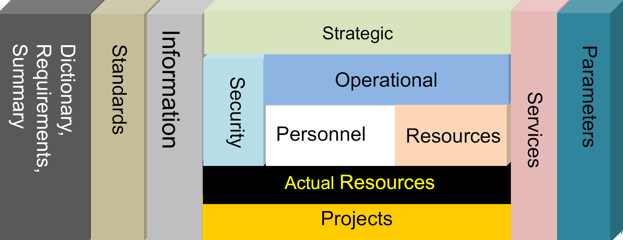
The framework proposes to decompose the architecture using different domains. Here are explanations for the main ones:
- Strategic: This domain defines the main Strategic Goals, expected Capabilities , Strategic Phases of the mission, project or Enterprise level. Finally, at this stage, it is possible to define the specific Measures of Effectiveness (MoE) to specify the required efficiency of the mission.
- Operational: This domain defines the operational structure and behavior, including identification of “Performer” Entities (Stakeholders) and their associated activities and actions to support the mission execution and completion of the overall capabilities.
- Services: This domain defines services to fulfill the capabilities. Services may be distributed over different stakeholders and systems.
- Resources: This domain defines different physical resources which contribute to the mission,. A resource can be composed of systems, natural resources, components, etc.
- Personnel: This domain defines human actors, their interactions, and organizational dependencies.
- Actual Resources: This domain defines a specific solution class which uses efficient collaboration between human actors and systems to realize the expected mission goals and associated capabilities.
- Project: This domain defines the project organization needed to execute the mission including the associated project roadmaps.
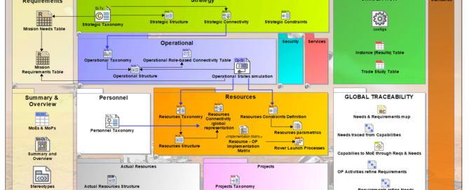
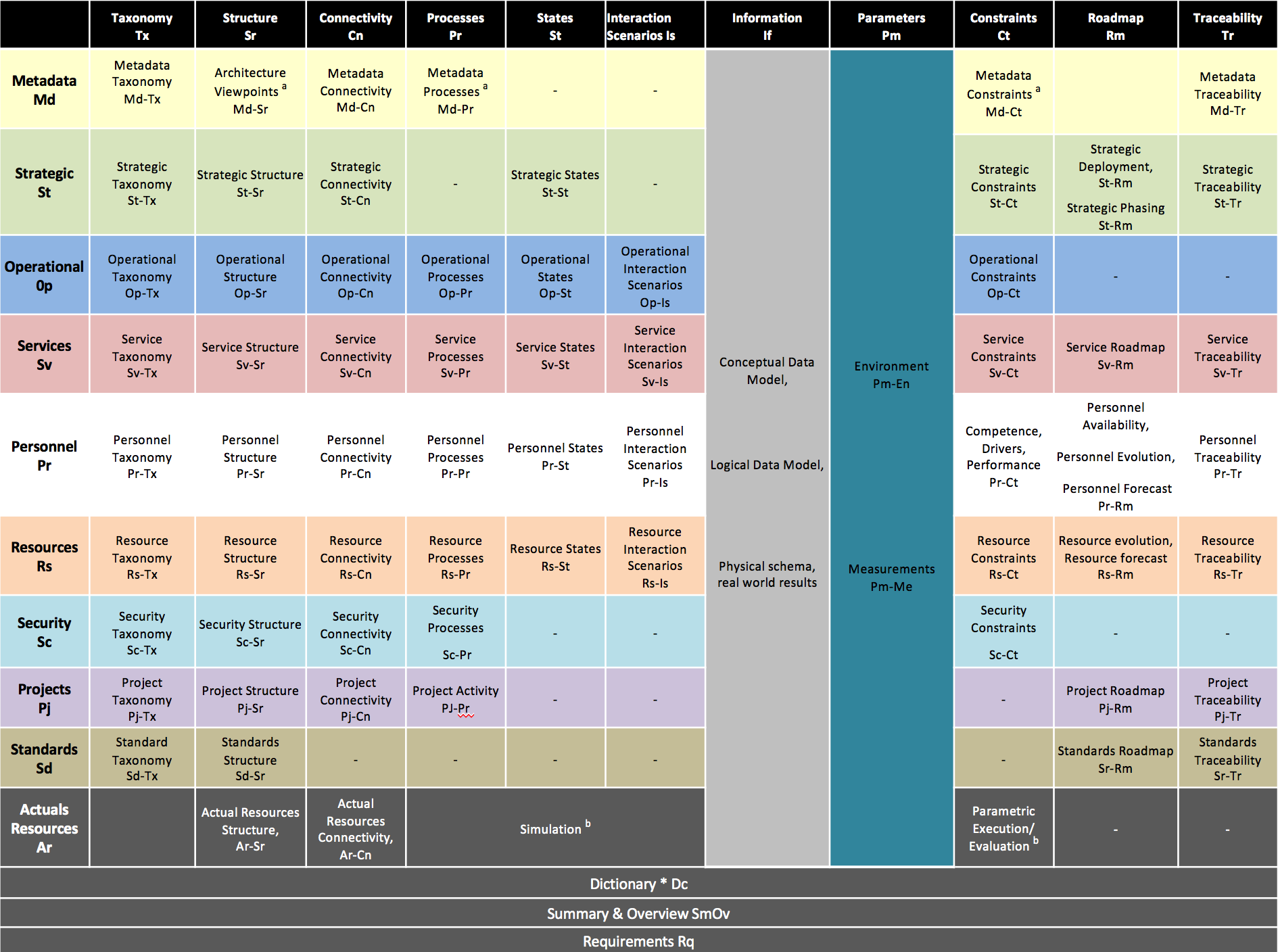
The modeling of these domains is supported by a “grid” view (from UAF V1.2 – Appendix C) illustrated below:
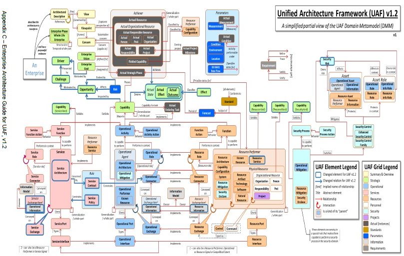
A simplified version of the related concepts (from UAF V1.2 – Appendix C) is presented below:
UAF vs SysML
In the context of Systems Modelling, there are other existing languages dedicated to the System of Interest definition (such as SysML, or ArcML).
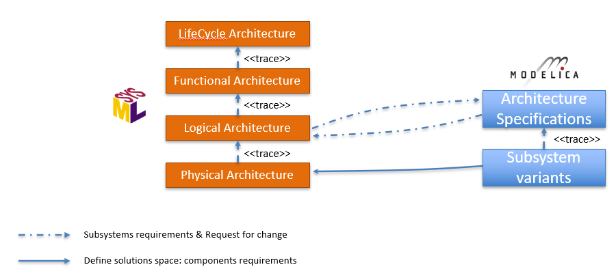
As stated before, implementations of UAF may be based on other language notations such as SysML, in particular when using UAFML, which is a SysML specialization (for example using the tool Magic System of Systems Architect). UAF has been designed to support Enterprise Architecture/Mission level and Systems interactions (with definitions for involved functions, resources and personnel), whereas SysML is a generic system definition language providing the key concepts and semantics for Requirements, Structure, Behavior and Parametric definitions. However, SysML on its own does not propose any specific structured framework (this should be completed by following a specific methodology).
As UAF is wide and proposes many concepts which might be complex or not useful for System of Interest definition, we suggest to limit the usage of UAF to the mission level as a support for Mission definition down until the selection of the System of Systems architecture and associated needs & requirements for each individual systems. Then, we recommend to use Systems Engineering languages completed with the appropriate methodology to perform definition of each System of Interest (SOI) using separation of concerns between Needs Analysis & Solutions.
When both enterprise and system-level perspectives are essential, UAFML and SysML can complement each other. UAFML provides the broader context, while SysML delves into the specific details.
In this article, we propose to address the definition of the Mission level (ConOps) with the UAF framework for the MARS exploration mission. Then, we will propose in a second article the definition of one of its systems (Exploration ROVER) using the SysML language and our internal Samares methodology and profile. Application on a case study – MARS Exploration mission
Mission Context
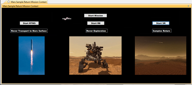
The Mars Exploration and Sample Return mission model developed using UAF is an example of how this framework can be applied to manage the complexity of a multi-system, multi-organization space project. The modeled mission is strongly inspired by the Mars 2020: Perseverance Rover and Mars Sample Return missions developed by the National Aeronautics and Space Administration and the European Space Agency. These missions are illustrated in the pictures below:
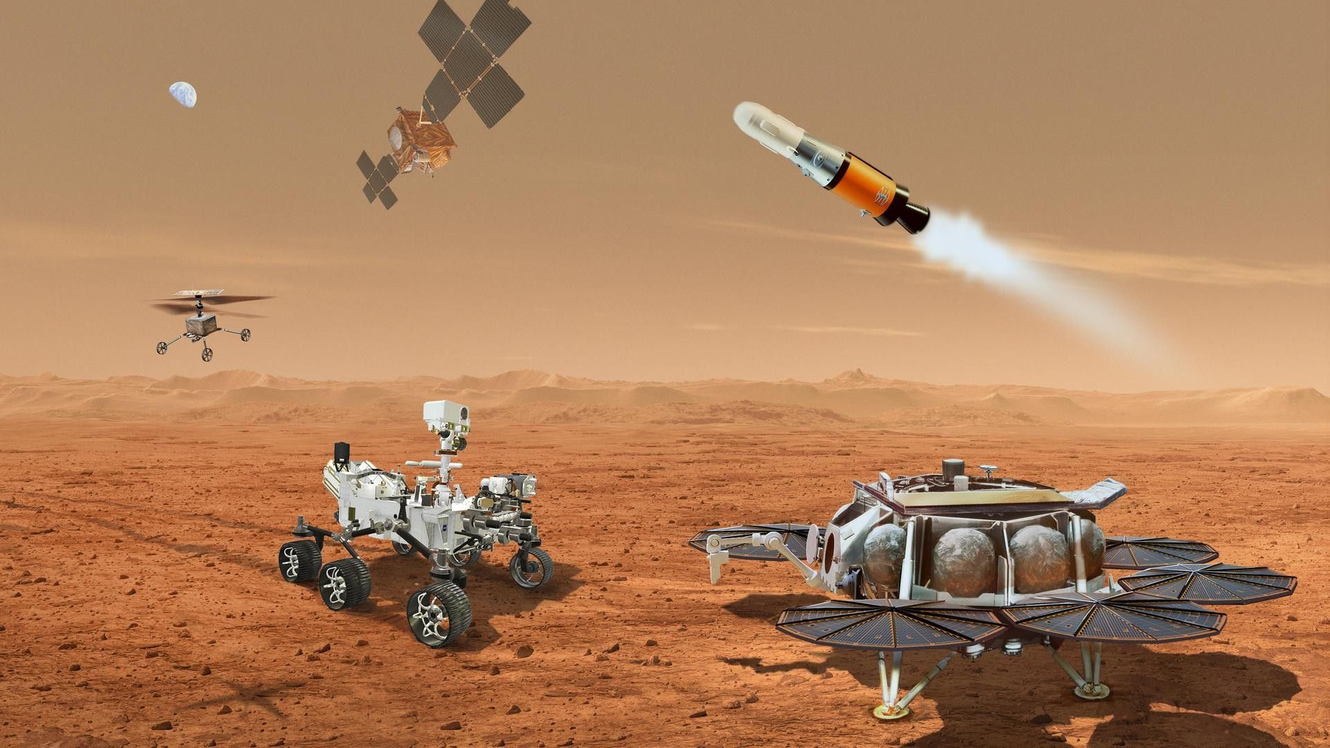
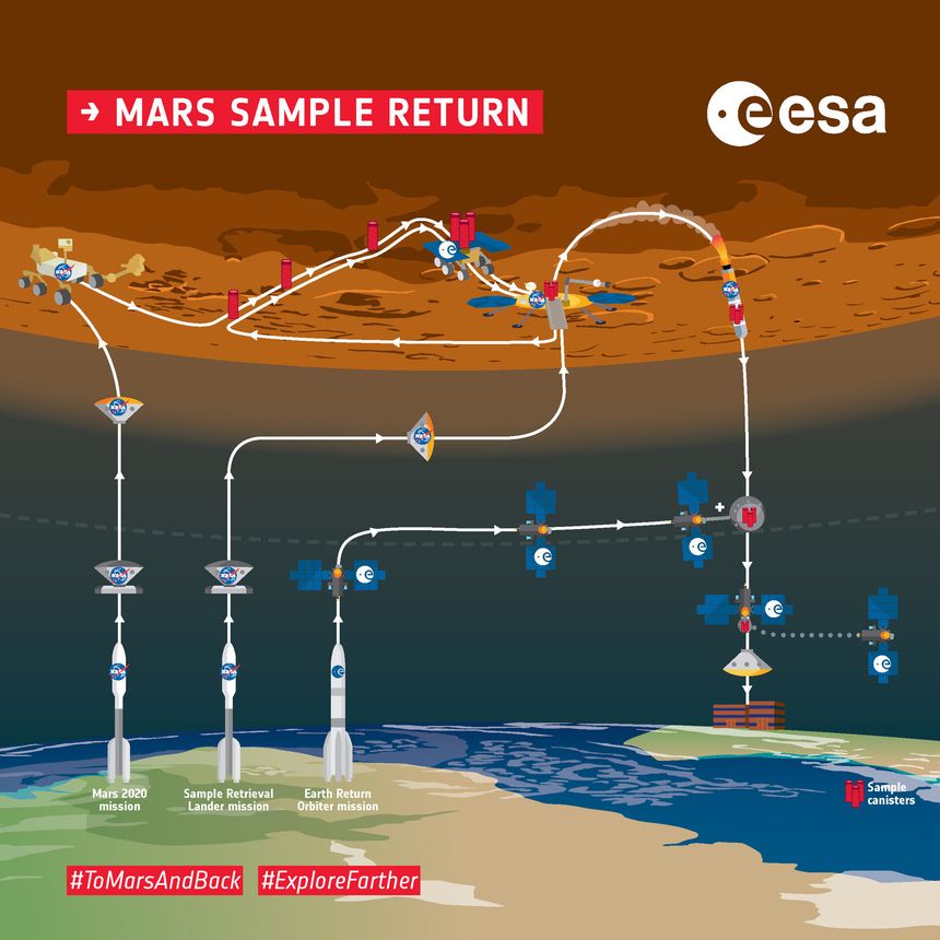
Both of these missions require collaboration between different space systems (Mars landing system, Orbiter, Perseverance Rover, Rocket, ..) and also with the Ground Operations systems operated by human actors to monitor and control the execution of the Mission.
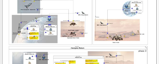
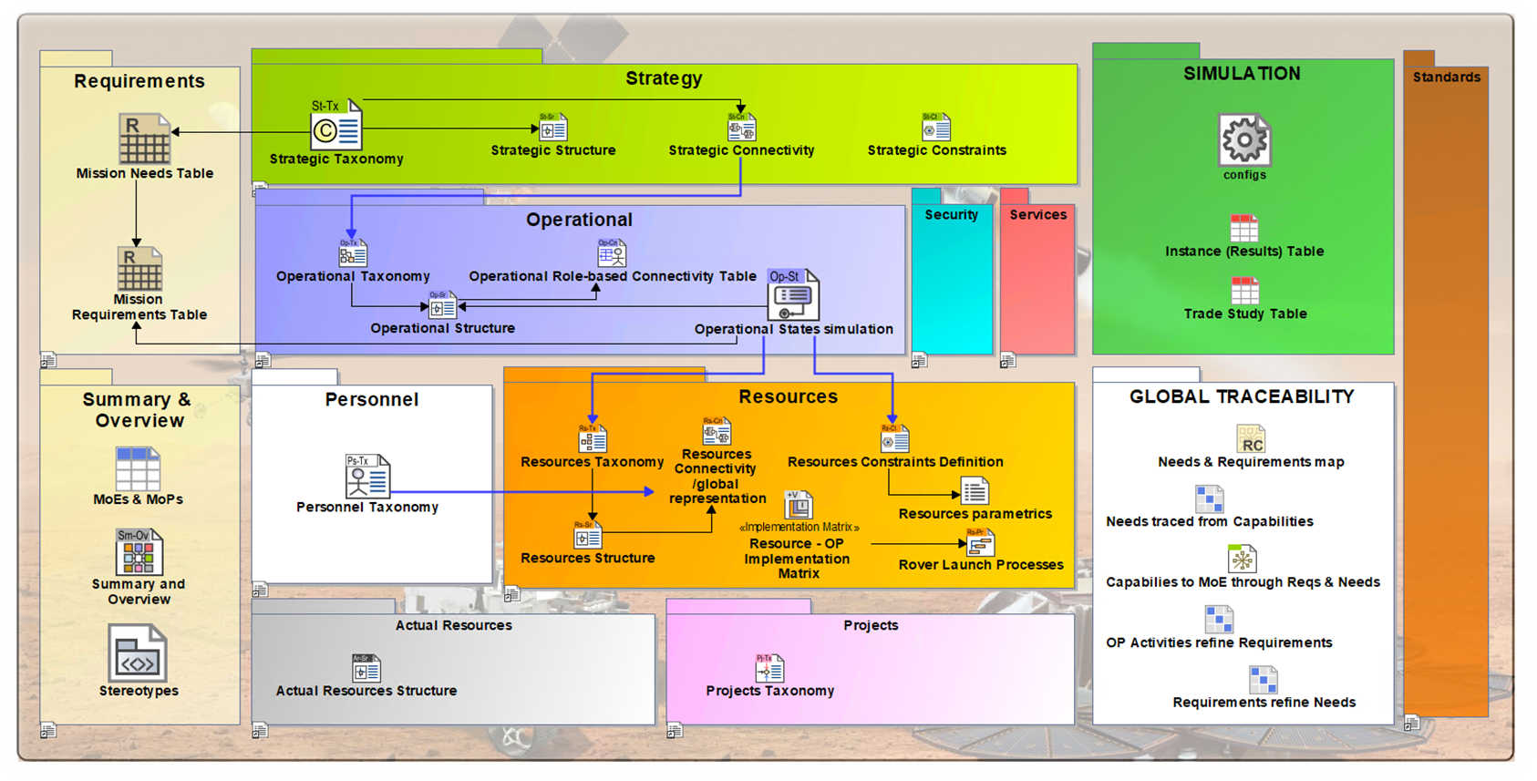
We apply UAF to the MARS Exploration mission and capture the main mission goals, expected mission efficiency, the contributions of the various systems and human actors involved, their interactions, and how they contribute to the overall mission objectives through the use of some of the proposed viewpoints as illustrated in the figure below:
Strategic Analysis
As stated in the UAF overview, the Strategic Analysis intends to define main strategic goals and expectations from the mission point of view. To perform this, we start by identifying the expected capabilities and associated relations with the Strategic Phases from the mission perspective:
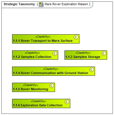
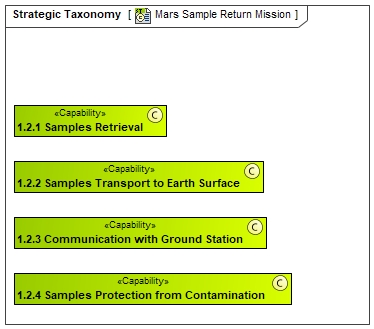
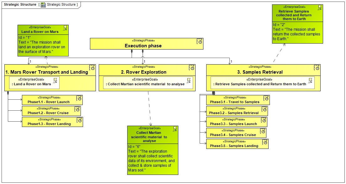
In these diagrams, we have decomposed the different capabilities expected from MARS Rover mission and Sample Retrieval defined as capabilities. Then, we have decomposed the mission in different strategic phases :
- For takeoff, travel and landing on Mars (context of ROVER Perseverance NASA Mission)
- For exploring the Mars surface using the Rover (context of ROVER Perseverance NASA Mission)
- For launching a new rocket and appropriate systems to retrieve samples on Mars and come back to earth. (context of Mars Sample Return ESA Mission)
In fact, Perseverance ROVER mission and Pars Sample return are 2 different missions but using some common systems (in particular ROVER). That is the reason why, we have decided to decompose them as 2 different phases (occuring at different time frame).
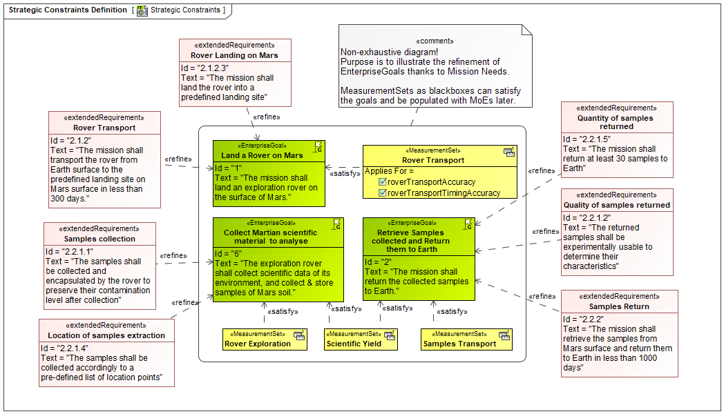
Finally we used the UAF Strategic Viewpoint to define some associated Measures of Effectiveness and define some requirements for specific capabilities as illustrated below:
Operational Architecture
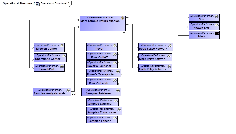
The Operational (Op) viewpoint intends to provide a description of the requirements, operational behavior, structure, and exchanges required to support (i.e., exhibit) the capabilities.
We first started with Operational Entities (Operational Performers) identification which contribute to the mission. It can be noticed that the identified performers are defined as generic entities and do not focus on their specific technology. We also define the interactions between entities:
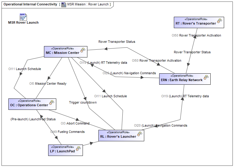
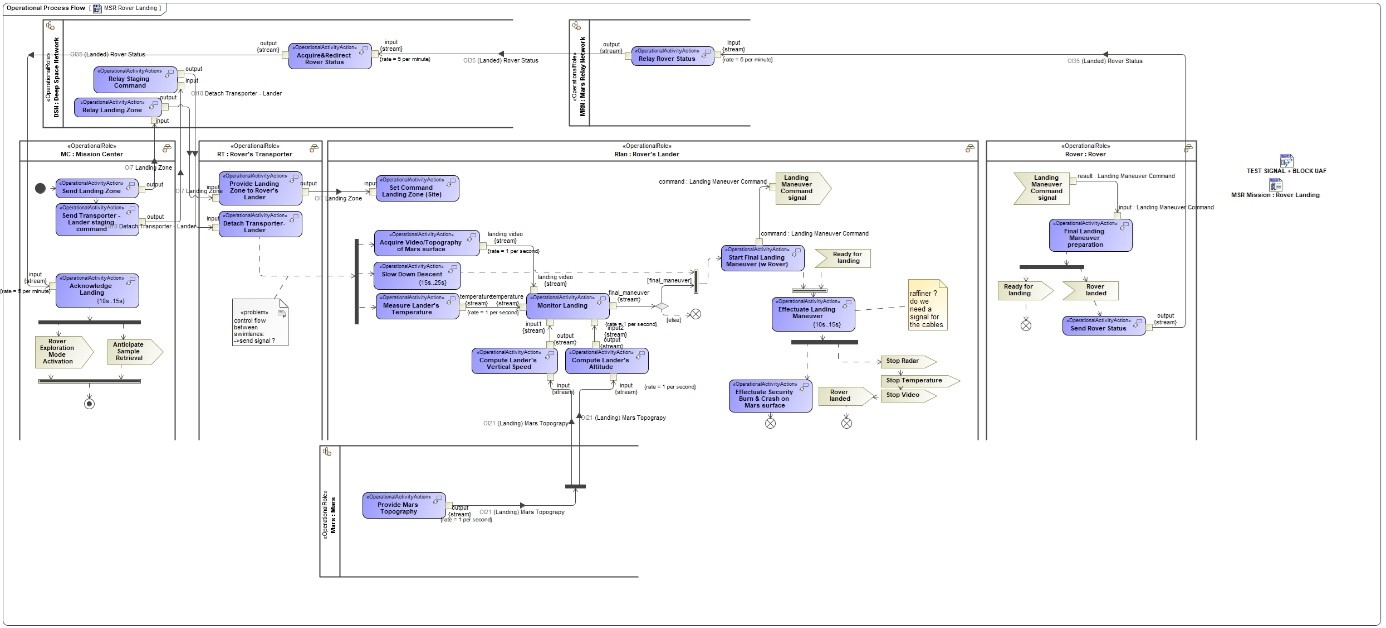
Then, we defined the associated Process flow involving the different Entities in the diagram below:
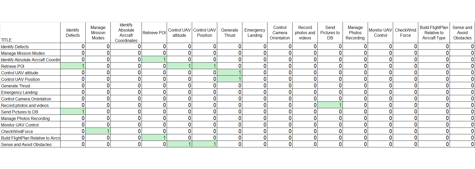
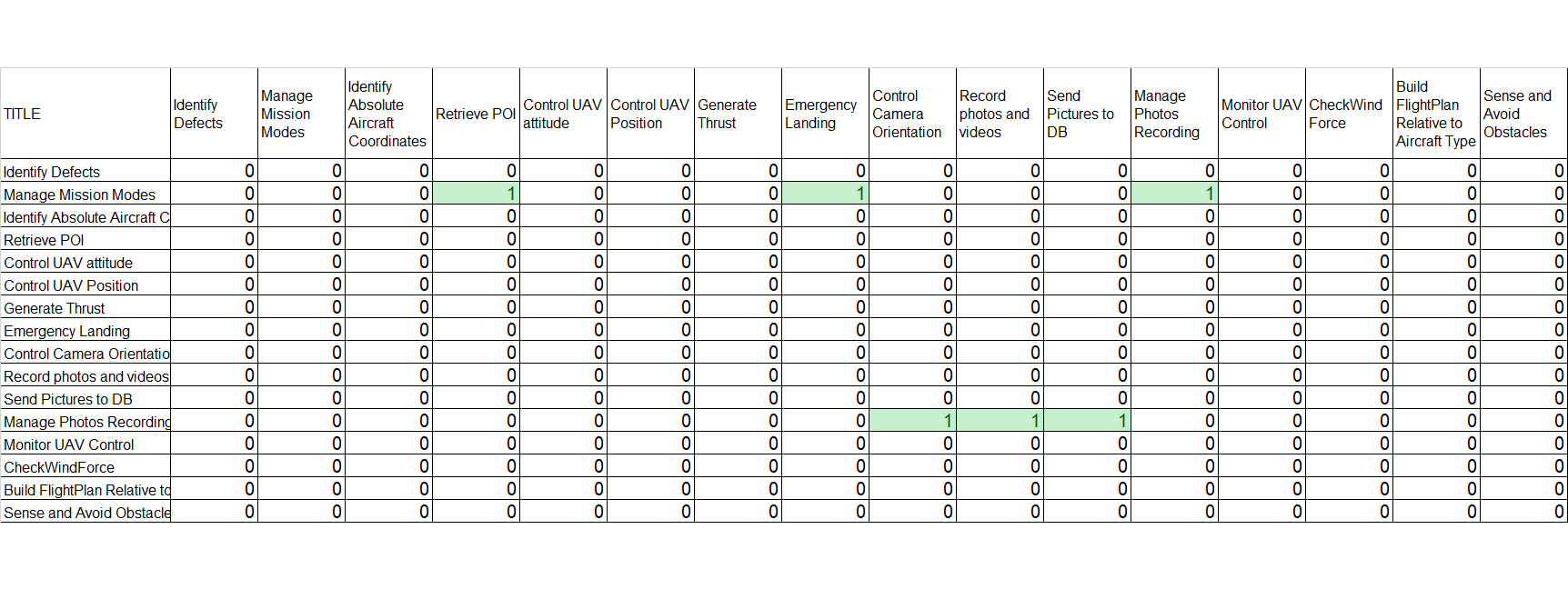
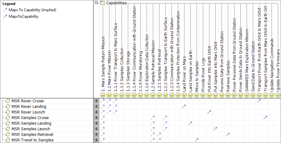
In order to verify the adequacy of these Process activities to support the defined capabilities, we established the following traceability matrix:
Resources Architecture
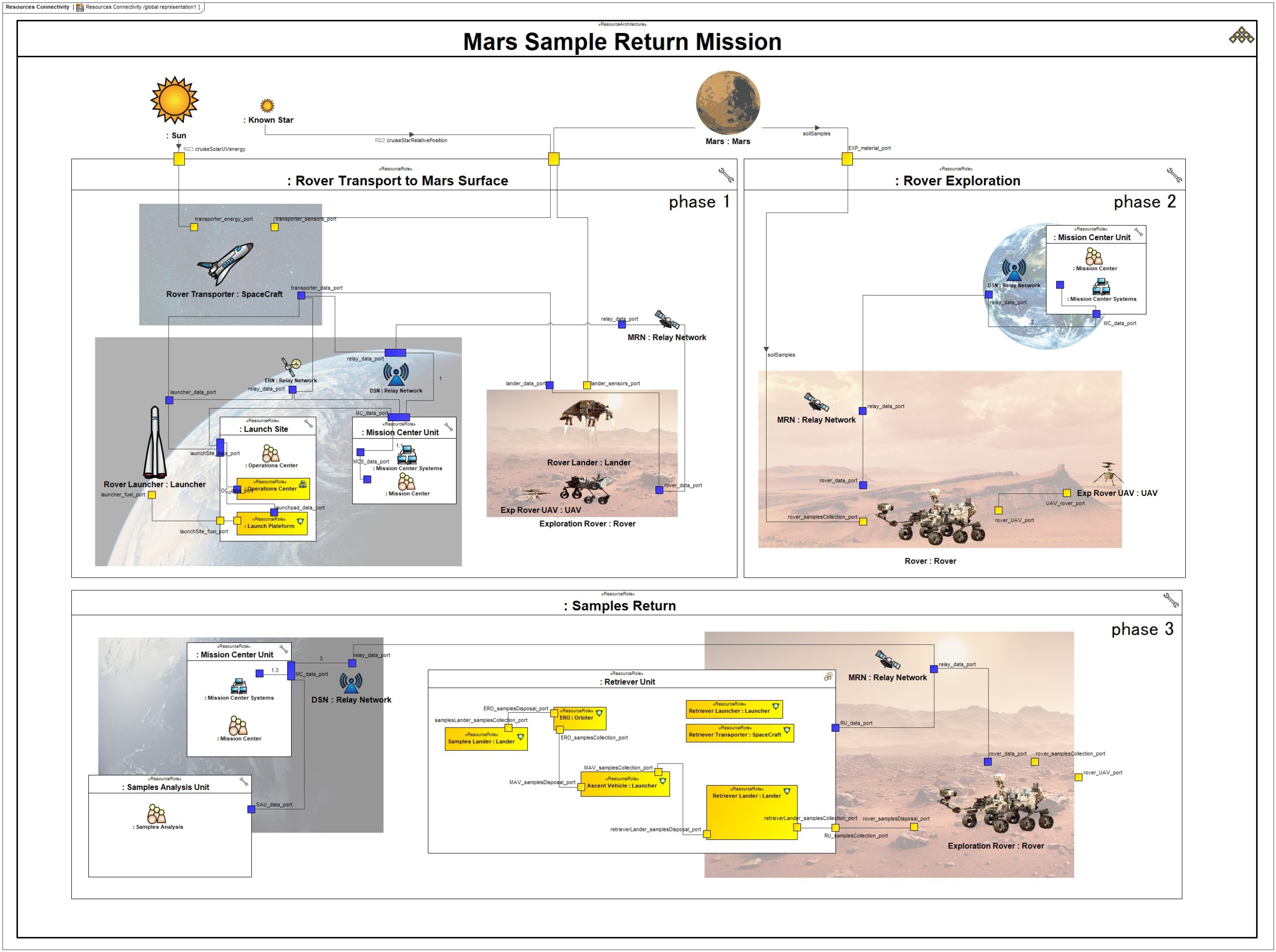
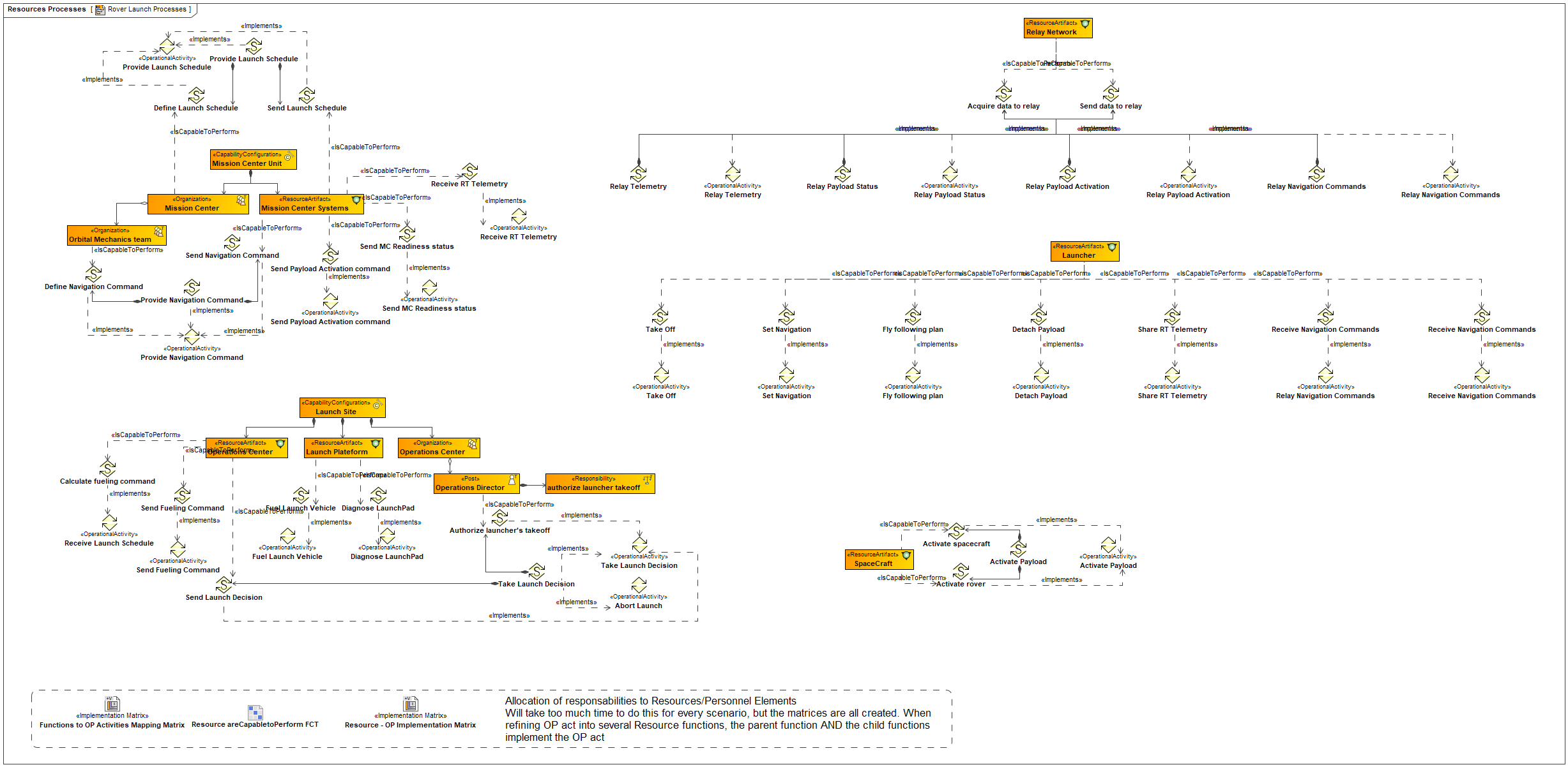
The Resources (Rs) domain intends to define the solution architectures to implement operational requirements. It captures a solution architecture consisting of resources, e.g. organizations, software, artifacts, capability configurations, natural resources. In our case study, we defined the physical structure and the expected systems interfaces of one of possible solution class:
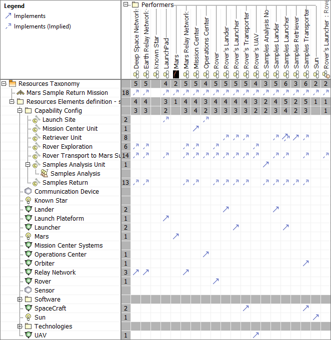
Then, we define the mapping between operational performers and Resources and also responsibility sharing between humans and physical resources (in particular for the Operations Center activities) :
Mission Requirements
As a result of this analysis, we established a requirement set for one of the specified systems – The Rover Transport – in the diagram below:
This requirement set will be used as the starting point to define the various Systems of Interest (SoI) that collaborate for this mission. Each of those SoI will start or adapt their definition to comply with this requirement set. They will use SysML based method and tools. This will be detailed in a future article.
Verification & Validation using Simulation
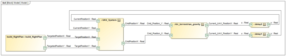
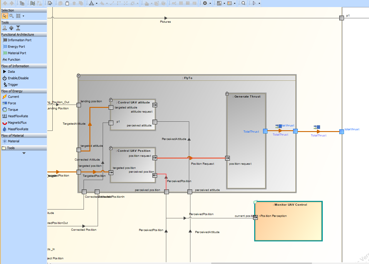
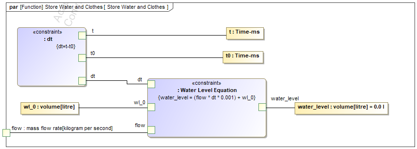
Once the architecture of the Mission is finalized, we can define the main physical equations and perform a tradeoff analysis to explore the performance of different solution classes. To do this, we established a Parametric diagram that can be seen below:
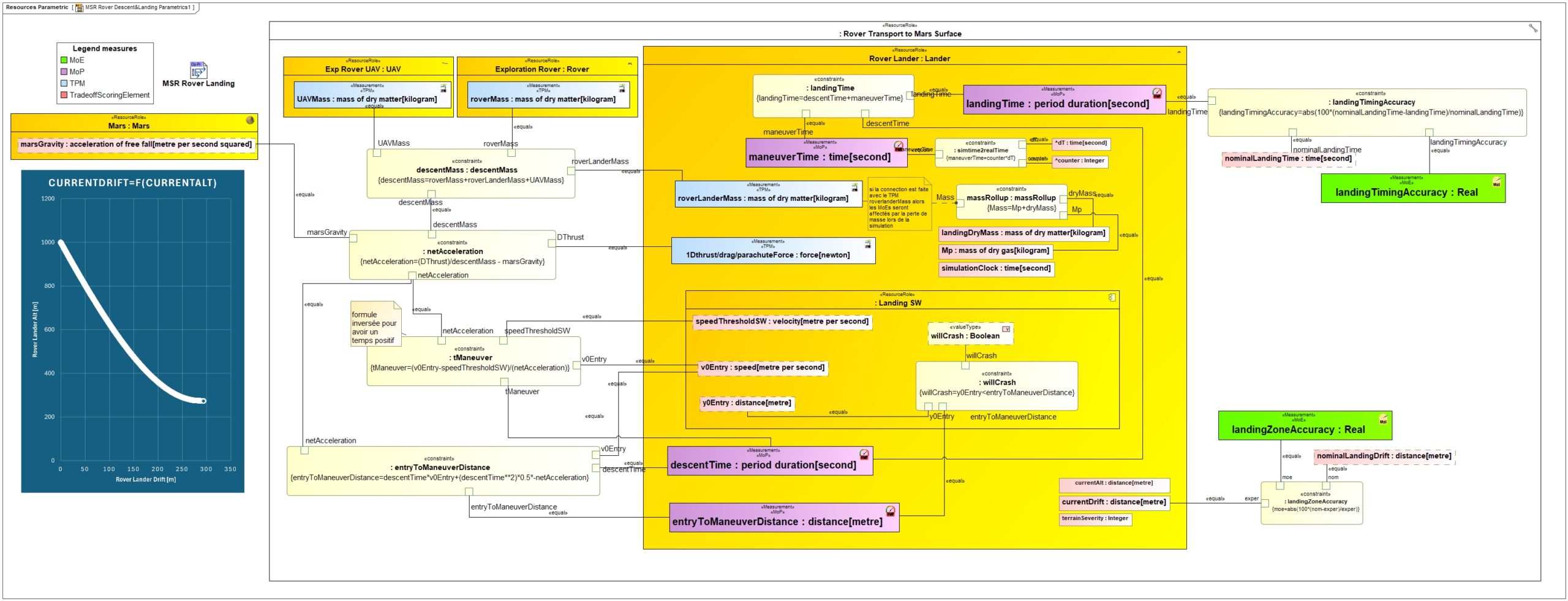
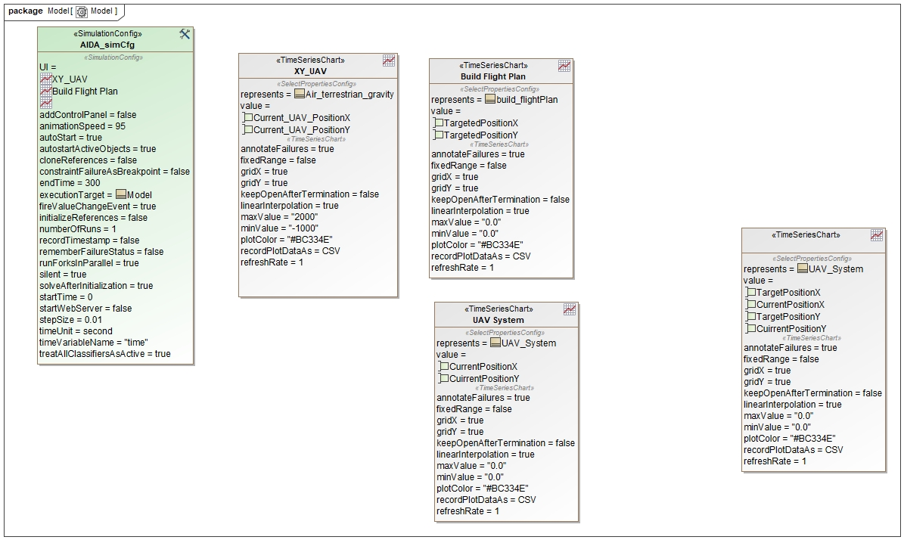
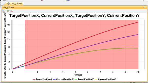
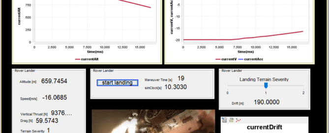
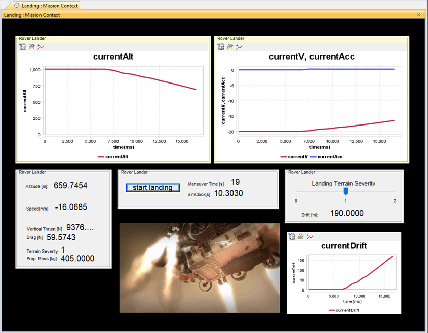
Then, we can define a specific Graphical User Interface to simulate the mission efficiency and visualize the results:
Conclusion and future work
With this article, we have illustrated the usage and benefits of UAF to define the Concept of Operations (ConOps), including the overall mission analysis which describes the collaboration between different systems to achieve a common goal. To complete this work, we would like to further explore the following things:
- Explore the benefit of additional UAF viewpoints, including Personnel, Services and Actual Resources.
- Complete the definition of Measures of Effectiveness (MoE) and their relations/equations with the System’s Measures of Performance (MoP)
- Perform Design Space Exploration using the MDA-MDO technique to define and assess the efficiency of different solution classes
- Trace our UAF model with a System of Interest model (Rover Exploration system)
Acknowledgements
We are very grateful to Louis Brial for his internship work and his contribution to this article and its associated contents.