Part 5 – Coupling optimization of logical architecture using genetic algorithm
This article is part of a monthly series entitled "Advanced MBSE with SysML and other languages".
In the first set of articles, this series explains how to use a modeling approach based on the SysML notation to progressively analyze, structure, refine and derive stakeholder needs and requirements into system architecture and lower-level requirements, down to configuration items containing software and hardware parts.
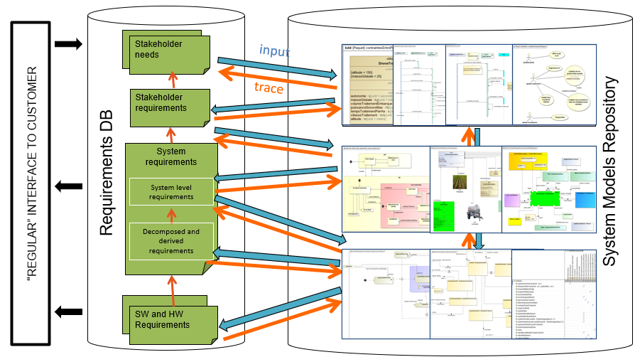
In the second set of articles, this series will focus on the links to other modeling languages used to detail the design and/or perform detailed analysis and simulations to evaluate, verify or validate the virtual representation of the system.
In the previous article, we explained how it is possible to define a Logical Architecture from a Functional architecture, using an allocation matrix between functions and logical components.
In this article, we go a step further by extracting the coupling metric between functions from the Functional Architecture (using an N² diagram technique) and using an optimization algorithm to minimize the coupling between logical components.
It is possible to consider several criteria with this method such as end to end latency requirements on interfaces. In this case, the algorithm tries to find the best solution that satisfies the coupling minimization, allocation constraints, and also timing constraints. In this article, we will focus on coupling minimization only.
Minimizing the coupling between components, a good systems engineering practice!
Among Systems Engineering best practices, as stated in many standards, it is key to minimize the coupling between the sub-systems in order to master the product complexity. For instance, in the IEC 61508:2000 we find:
"The interfaces between subsystems are kept as simple
as possible and the cross-section (i.e. shared data, exchange of information) is minimised.".IEC 61508:2000 – Functional safety of electrical/electronic/
programmable electronic safety-related systems – Part 7:
Overview of techniques and measures
Are there any techniques or methods to support systems architects in minimizing the coupling between components?
Yes, to achieve such minimization, a well-known method consists of using Coupling Matrices (also called N 2 diagrams) and then reorganize them to identify architectures with minimal coupling.
Let us first explain how an N² diagram is defined, and let us illustrate that explanation with a case study. Secondly we will focus on the computation of the N² diagram to identify coupling optimization.
The coupling between components concerns the dependencies between the components. As explained in the previous article (part 4), the dependencies between the logical components mainly stem from the functional interfaces. So it is no surprise that we first start with the functional dependencies, use them to compute a coupling metric, and finally suggest an allocation of functions to components that minimizes the coupling.
Introduction to the N² diagram method
The N 2 chart, also referred to as N 2 diagram, N-squared diagram or N-squared chart, is a diagram in the shape of a matrix, representing functional or physical interfaces between system elements. It is used to systematically identify, define, tabulate, design, and analyze functional and physical interfaces. It applies to system interfaces and hardware and/or software interfaces.
[2] Wikipedia: https://en.wikipedia.org/wiki/N2_chart
In the previous article, we explained how it is possible to define a Logical Architecture from a Functional architecture, using an allocation matrix between functions and logical components.
Here below is an example of an N² diagram for a project with 9 functions that have dependencies.
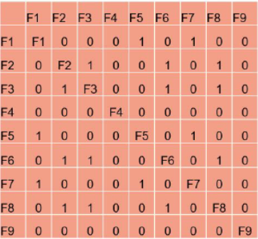
In this matrix, the "1" represents an existing interface between the function of the concerned row and the function of the concerned column. The "0" indicates that there is no relation between those functions. In this example the matrix is symmetric, indicating that all the links are bi-directional. This is not the standard rules of the N² chart, which are better explained by the following figure.
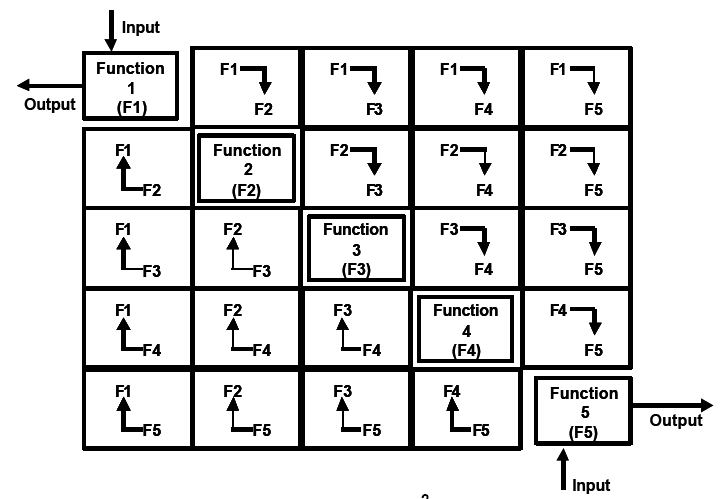
Illustration of how to read an N² diagram
The placement of the "1" (above or below the diagonal) determines which function is the source and which function is the target of the link.
The use of a coupling matrix is mentioned by the INCOSE SE handbook as a useful practice :
Coupling matrices (also called N 2 diagrams) are a basic method to define the aggregates and the order of integration (Grady, 1994). They are used during architecture definition, with the goal of keeping the interfaces as simple as possible… Simplicity of interfaces can be a distinguishing characteristic and a selection criterion between alternate architectural candidates. The coupling matrices are also useful for optimizing the aggregate definition and the verification of interfaces.
Systems Engineering Handbook 4th edition 2015 in chapter 4.4.2.6 Coupling matrix
From this matrix we can compute a coupling value regarding the interfaces defined between the Logical Components (deduced from the interfaces between functions allocated to these components). The coupling value represent an evaluation of the coupling complexity between logical components based on the following formula derivated from software coupling metrics in Dhama, "Quantitative models of cohesion and coupling in software", Journal of Systems and Software vol; 29, Apr, 1995
where the parameters are defined as follows:
- `M_(k)`: logical component under consideration
- `d_(i)`: number of input data parameters
- `c_(i)`: number of input control parameters
- `d_(o)`: number of ouput data parameters
- `c_(o)`: number of ouput control parameters
- `w`: number of modules called (fan-out)
- `r`: number of calling the module under consideration (fan-in)
Now, let us see an illustration on a case study.
A sample case to illustrate the definition and use of the N² diagram
Our sample case is based on a case study elaborated within IRT St-Exupery called AIDA (Aircraft Inspection by Drone Assistant). This example was initially developed in a Capella environment and is available at https://sahara.irt-saintexupery.com/AIDA/AIDAArchitecture. For this article, we have translated the sample case to the SysML language.
In the previous article (part 4), we used this sample case to show how we can initialize the logical architecture from the functional architecture with the use of an allocation matrix between functions and logical components. In this article, we use it again, but this time we explain how to use optimization techniques to determine automatically the "best fit" to minimize the coupling. In other words, we want to define one or several possible allocations (illustrated by allocation matrices) between functions and logical components that minimize the coupling between the components.
Let us see this in practice.
N² diagram from the Functional Architecture
In the previous article (part 4) we showed a possible functional architecture elaborated for this sample case. We recall it in the figure below:
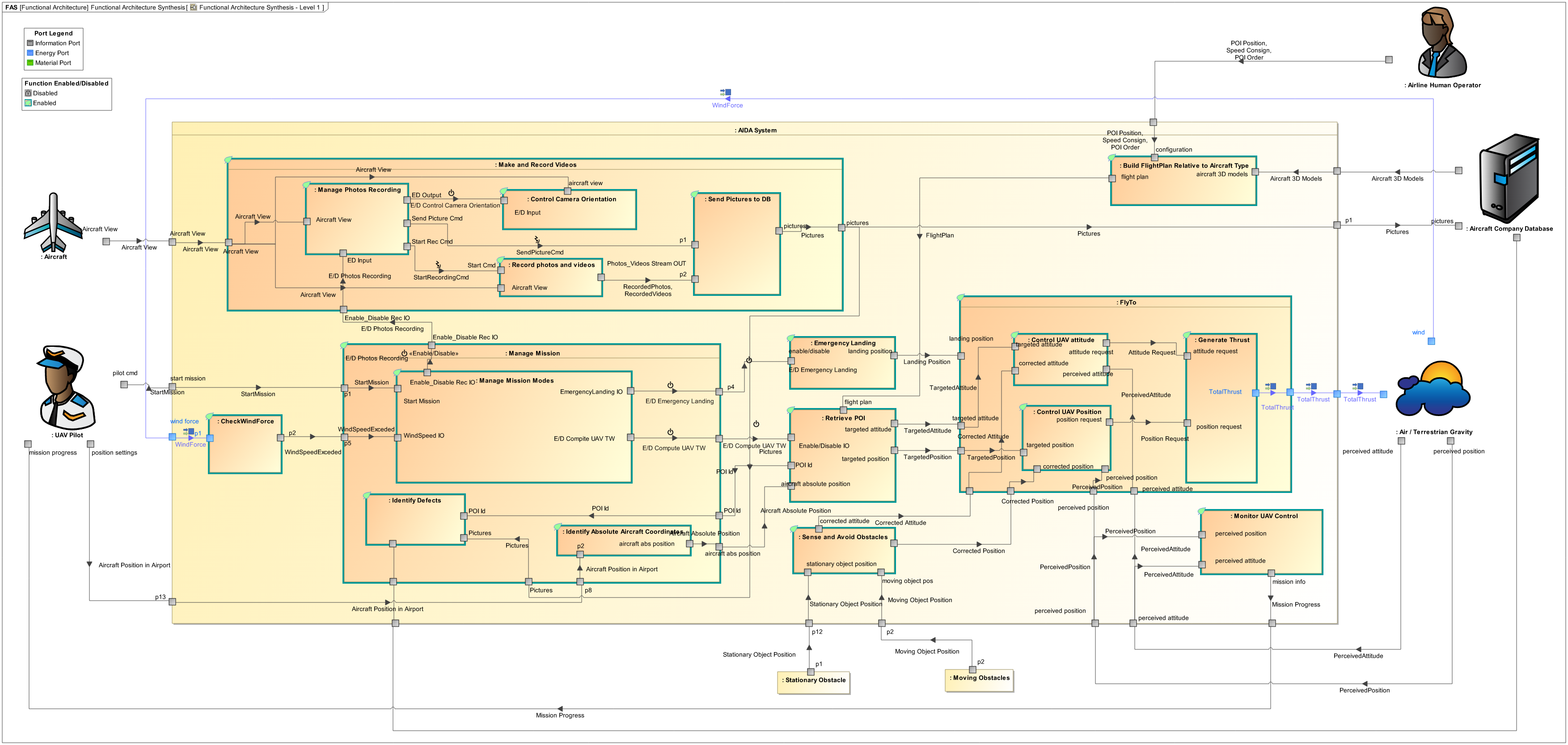
For this functional architecture, we can extract 2 N 2 diagrams for the leaf functions by analyzing their dependencies:
- Data/energy/material flows
- Control (Enable/Disable or Trigger) flows
The results are displayed in the 2 figures below:
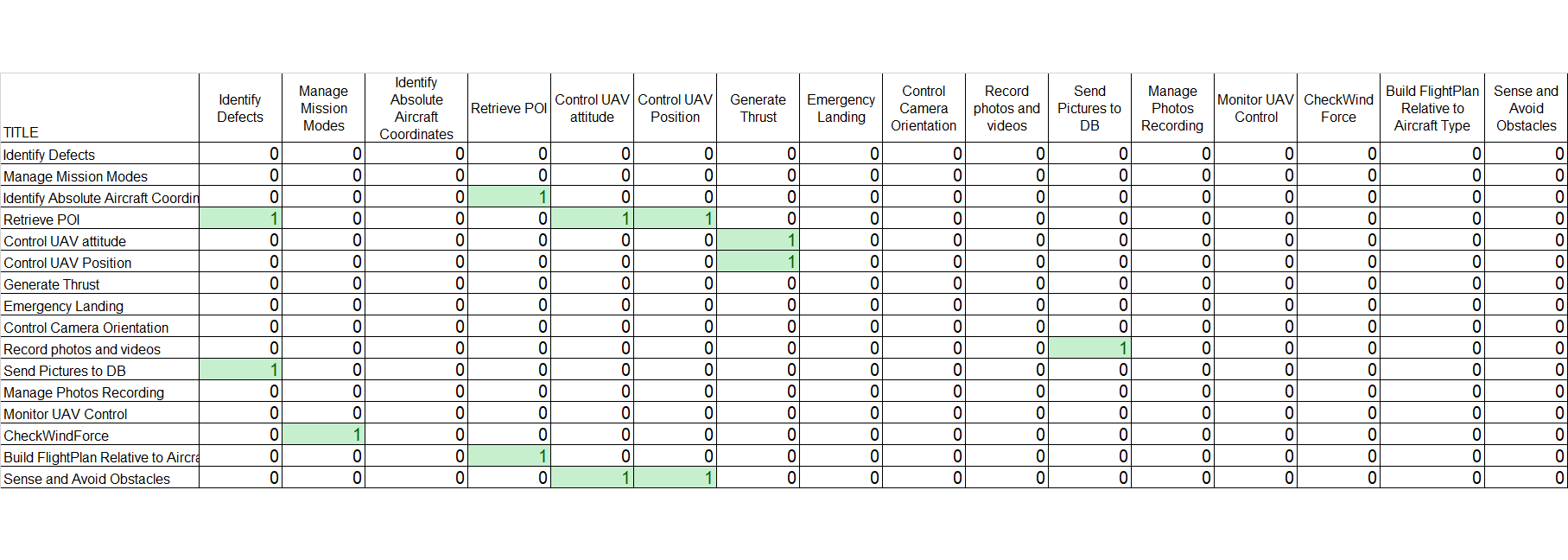
N² matrix for data/energy/material flow
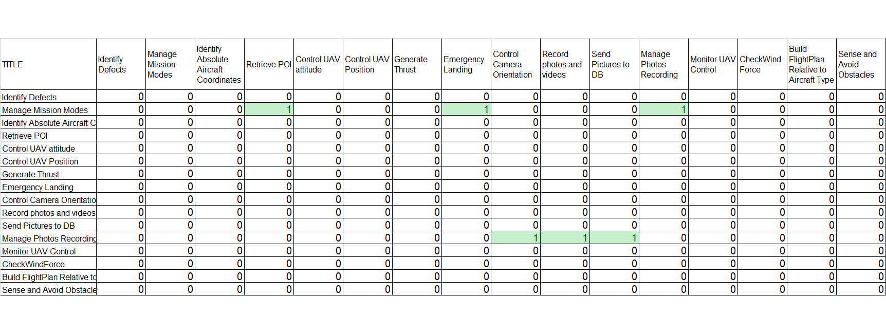
N² matrix for control flow
Now we want to define a logical architecture that minimizes the number of interfaces between its subsystems.
Optimization of allocation between functions and logical components
From a functional N² diagram to a logical architecture…
To perform optimization between components, we analyze the functions to functions coupling matrices introduced previously and we use them as input for a genetic algorithm presented later in this article. This algorithm will progressively iterate over different possible logical architectures and will calculate the coupling between components. In the end, it will select the architectures that minimizes the coupling metric.
Let us look at a possible logical architecture. How do we define it? We simply define the components (or modules) as groups (or partitions) of functions.
As an example, in the figure below, the orange color part of the figure illustrates an allocation (or partition) strategy of the 9 functions into 3 modules: M1, M2, and M3. In this figure, we are not interested in the internal structure of each module, which is why we do not represent the functional interfaces between functions of the same module. However, we want to see the functional interfaces between functions allocated to different modules because it will give us the logical interfaces. If we focus on the M3 module, we see in green the M3 inputs, and in blue the M3 outputs.
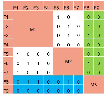
Example of coupling analysis for 3 modules (green highlight on Module 3 inputs, blue highlight on Module 3 outputs)
Note: we recommend reading the previous article for more details on the relationships between the functional architecture and the logical architecture.
From this matrix with modules, we can now compute a coupling metric regarding the interfaces of the modules.
Using a Genetic Algorithm to optimize the allocation of functions
Genetic algorithms are algorithms inspired by evolutionary principles. The main purpose of this kind of algorithm is to explore the solution space of a problem in order to satisfy a set of criteria. The general principles of genetic algorithms are illustrated on the Figure below.
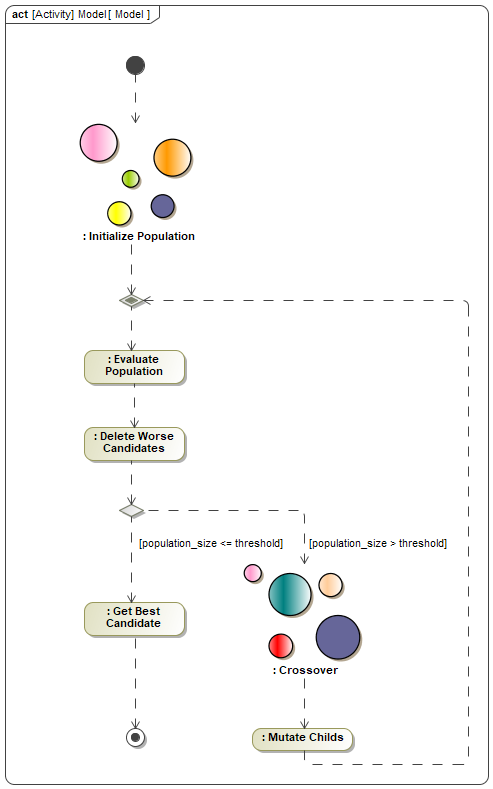
Genetic Algorithm Process
The first step is to create randomly a set of initial subjects (1). This set is called the initial population. The initial population is composed of subjects each representing a possible set of functions allocations. Then, the algorithm evaluates each subject using a fitness function (2). This function makes it possible to give a value, or a rank, to a subject, to estimate its proximity with the "optimal" solution. In our case the fitness function is the coupling equation C. The candidates that are too far from the desired solution are deleted (3).
Then the algorithm evaluates the number of remaining subjects. For instance, if the population size is less or equal to 4, then the algorithm returns the best solution amongst the 4 remaining subjects. On the contrary, if the population size is greater than a specific threshold, then the algorithm continues. And this is where things become interesting…
Here begins the core biomimicry part of the genetic algorithm: the remaining subjects cross over, i.e. they exchange their genes to produce new subjects (4). Finally, the newly created childs are subject to mutation (5): part of their characteristics randomly change. Cross over and mutation are usefull to stay away from local optimum by spreading new subjects through the solution space.
Genetic algorithms are configurable using the following set of parameters:
- Initial population size – a key parameter to ensure enough coverage of the solution space at the begining
- Max generation number – parameter to ensure that the algorithm ends even if the population grows.
- Percentage of survivor – the percentage of the worst subjects to delete
- Percentage of parents – the percentage of subjects that cross over
- Percentage of child to mutate – the percentage of new subjects to mutate after the cross over
- Percentage of gene to mutate – the percentage of genes to mutate for each new subject
What about constraints on allocations?
In practice, systems engineers already have good ideas of some allocations between functions and components or have constraints that exist on fixed allocations (for different reasons including security, performance…). So the genetic algorithm shall consider these first predefined allocations.
We have defined our genetic algorithm to be able to take as input a predefined partial allocation matrix with existing constraints. These constraints are considered by the algorithm that will then define possible logical architectures respecting the given constraints.
Selection of the "best" logical architecture that minimizes coupling
The genetic algorithm presented previously gives us one or several possible logical architectures that minimize the coupling between components while conforming to the functional architecture and eventual allocation constraints. We can use the results to generate or complete the allocation matrix between our functions and the components as presented below.
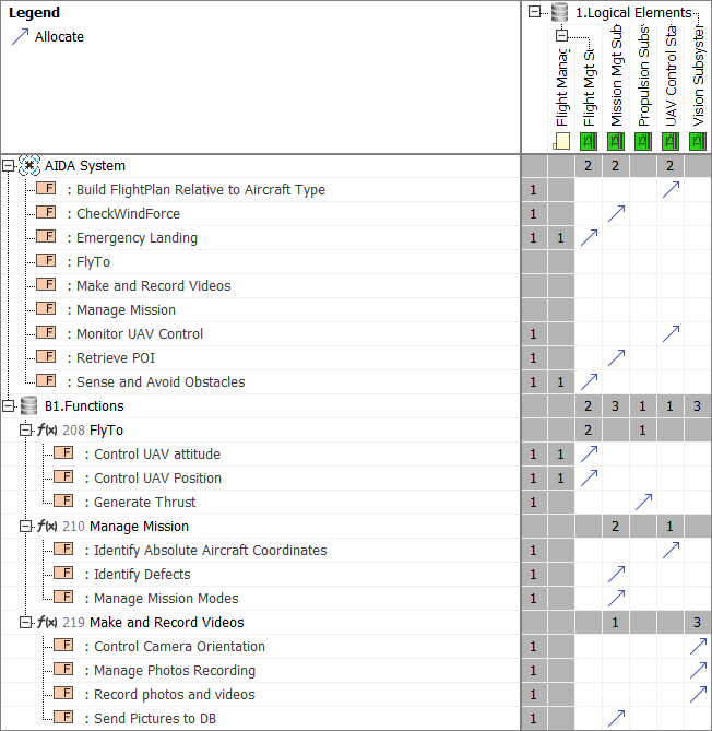
Allocation Matrix
Thanks to the completion of this allocation matrix, we can deduce a logical architecture, as explained in the previous article (part 4) that shows the different logical subsystems with their allocated functions and keeps the functional flows coming from the functional architecture.
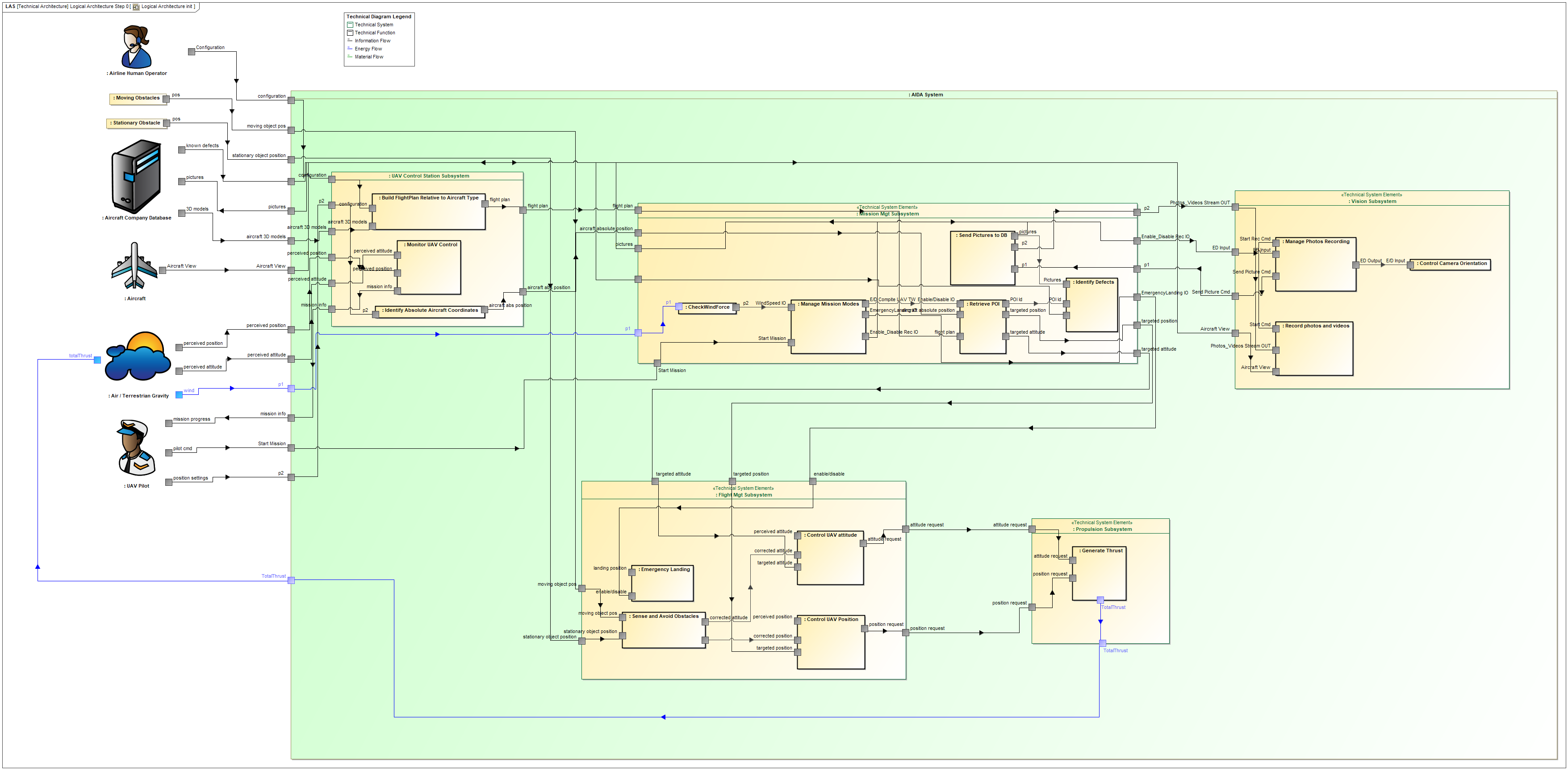
Logical architecture after allocation of functions using GA
Can we automate some of the steps presented above?
Yes!
At Samares Engineering, we have investigated automation of the different following steps :
- Extracting the initial N² Matrix from the functional architecture (for both data/energy/material and control flows)
- Exploring candidate logical architectures (functional to logical allocation) to automatically find the candidate architectures where the coupling metric is at a minimum value using the genetic algorithm.
- Defining allocation constraints (for example UAV control position function can be forced to be allocated to the Flight Control System).
Enjoy MBSE!
Acknowledgements
We are warmly gratefull to Yash Khetan and Minghao Wang for their contribution. It was great to work with both of you. See you!
Next articles to come…
- September 2020 – Digital continuity between SysML and Simulink
- October 2020 – Digital continuity between SysML and AADL
- November 2020 – Digital continuity between SysML and Modelica
- January 2021 – Co-simulation of SysML and other models through FMI
Previous articles in the series
- April 2020 – Formalization of functional requirements
- May 2020 – Derivation of requirements from models: From DOORS to SysML to DOORS again
- June 2020 – Early validation of stakeholder needs through functional simulation
- July 2020 – Consistency between functional and logical architectures